Science Practice Test 1 (Untimed) – Outschool

Item 1

Aging is a complex biological process that scientists are still working to fully understand. Two scientists propose differing explanations for the primary cause of aging in organisms.

Scientist 1

Aging occurs primarily due to progressive telomere shortening, which limits cellular replication. Telomeres are repetitive DNA sequences at the ends of chromosomes that protect genetic material during cell division. However, with each replication, telomeres shorten because DNA polymerase cannot fully replicate the lagging strand.

Once telomeres reach a critically short length, cells enter a state called replicative senescence, where they cease dividing. This loss of cellular function contributes to tissue degeneration and organismal aging. Studies show that species with longer telomeres tend to live longer, and in certain experiments, mice engineered to express higher telomerase activity (an enzyme that elongates telomeres) exhibit extended lifespans.

Scientist 2

Aging is driven by cumulative molecular damage caused by reactive oxygen species (ROS), metabolic byproducts, and external environmental factors. Over time, these oxidative stressors damage cellular components, including DNA, proteins, and lipids. Unlike telomere shortening, which affects cell division, this model suggests that aging is due to an increasing burden of irreparable intracellular damage that impairs normal function.

In experiments, organisms exposed to high levels of ionizing radiation and environmental toxins exhibit premature aging, even if their telomere length remains unchanged. Conversely, studies on caloric restriction and antioxidant treatments show that reducing oxidative stress can significantly extend lifespan. This suggests that aging results from an imbalance between damage accumulation and cellular repair mechanisms.

Which of the following best describes the key difference between the two scientists’ explanations of aging?

Item 2

Aging is a complex biological process that scientists are still working to fully understand. Two scientists propose differing explanations for the primary cause of aging in organisms.

Scientist 1

Aging occurs primarily due to progressive telomere shortening, which limits cellular replication. Telomeres are repetitive DNA sequences at the ends of chromosomes that protect genetic material during cell division. However, with each replication, telomeres shorten because DNA polymerase cannot fully replicate the lagging strand.

Once telomeres reach a critically short length, cells enter a state called replicative senescence, where they cease dividing. This loss of cellular function contributes to tissue degeneration and organismal aging. Studies show that species with longer telomeres tend to live longer, and in certain experiments, mice engineered to express higher telomerase activity (an enzyme that elongates telomeres) exhibit extended lifespans.

Scientist 2

Aging is driven by cumulative molecular damage caused by reactive oxygen species (ROS), metabolic byproducts, and external environmental factors. Over time, these oxidative stressors damage cellular components, including DNA, proteins, and lipids. Unlike telomere shortening, which affects cell division, this model suggests that aging is due to an increasing burden of irreparable intracellular damage that impairs normal function.

In experiments, organisms exposed to high levels of ionizing radiation and environmental toxins exhibit premature aging, even if their telomere length remains unchanged. Conversely, studies on caloric restriction and antioxidant treatments show that reducing oxidative stress can significantly extend lifespan. This suggests that aging results from an imbalance between damage accumulation and cellular repair mechanisms.

Which of the following findings would most strongly challenge Scientist 1’s hypothesis?

Item 3

Aging is a complex biological process that scientists are still working to fully understand. Two scientists propose differing explanations for the primary cause of aging in organisms.

Scientist 1

Aging occurs primarily due to progressive telomere shortening, which limits cellular replication. Telomeres are repetitive DNA sequences at the ends of chromosomes that protect genetic material during cell division. However, with each replication, telomeres shorten because DNA polymerase cannot fully replicate the lagging strand.

Once telomeres reach a critically short length, cells enter a state called replicative senescence, where they cease dividing. This loss of cellular function contributes to tissue degeneration and organismal aging. Studies show that species with longer telomeres tend to live longer, and in certain experiments, mice engineered to express higher telomerase activity (an enzyme that elongates telomeres) exhibit extended lifespans.

Scientist 2

Aging is driven by cumulative molecular damage caused by reactive oxygen species (ROS), metabolic byproducts, and external environmental factors. Over time, these oxidative stressors damage cellular components, including DNA, proteins, and lipids. Unlike telomere shortening, which affects cell division, this model suggests that aging is due to an increasing burden of irreparable intracellular damage that impairs normal function.

In experiments, organisms exposed to high levels of ionizing radiation and environmental toxins exhibit premature aging, even if their telomere length remains unchanged. Conversely, studies on caloric restriction and antioxidant treatments show that reducing oxidative stress can significantly extend lifespan. This suggests that aging results from an imbalance between damage accumulation and cellular repair mechanisms.

Scientist 2 would most likely predict that which of the following interventions could extend lifespan?

Item 4

Aging is a complex biological process that scientists are still working to fully understand. Two scientists propose differing explanations for the primary cause of aging in organisms.

Scientist 1

Aging occurs primarily due to progressive telomere shortening, which limits cellular replication. Telomeres are repetitive DNA sequences at the ends of chromosomes that protect genetic material during cell division. However, with each replication, telomeres shorten because DNA polymerase cannot fully replicate the lagging strand.

Once telomeres reach a critically short length, cells enter a state called replicative senescence, where they cease dividing. This loss of cellular function contributes to tissue degeneration and organismal aging. Studies show that species with longer telomeres tend to live longer, and in certain experiments, mice engineered to express higher telomerase activity (an enzyme that elongates telomeres) exhibit extended lifespans.

Scientist 2

Aging is driven by cumulative molecular damage caused by reactive oxygen species (ROS), metabolic byproducts, and external environmental factors. Over time, these oxidative stressors damage cellular components, including DNA, proteins, and lipids. Unlike telomere shortening, which affects cell division, this model suggests that aging is due to an increasing burden of irreparable intracellular damage that impairs normal function.

In experiments, organisms exposed to high levels of ionizing radiation and environmental toxins exhibit premature aging, even if their telomere length remains unchanged. Conversely, studies on caloric restriction and antioxidant treatments show that reducing oxidative stress can significantly extend lifespan. This suggests that aging results from an imbalance between damage accumulation and cellular repair mechanisms.

Suppose an experiment found that a population of fruit flies with artificially extended telomeres exhibited no significant increase in lifespan. What conclusion would this best support?

Item 5

Aging is a complex biological process that scientists are still working to fully understand. Two scientists propose differing explanations for the primary cause of aging in organisms.

Scientist 1

Aging occurs primarily due to progressive telomere shortening, which limits cellular replication. Telomeres are repetitive DNA sequences at the ends of chromosomes that protect genetic material during cell division. However, with each replication, telomeres shorten because DNA polymerase cannot fully replicate the lagging strand.

Once telomeres reach a critically short length, cells enter a state called replicative senescence, where they cease dividing. This loss of cellular function contributes to tissue degeneration and organismal aging. Studies show that species with longer telomeres tend to live longer, and in certain experiments, mice engineered to express higher telomerase activity (an enzyme that elongates telomeres) exhibit extended lifespans.

Scientist 2

Aging is driven by cumulative molecular damage caused by reactive oxygen species (ROS), metabolic byproducts, and external environmental factors. Over time, these oxidative stressors damage cellular components, including DNA, proteins, and lipids. Unlike telomere shortening, which affects cell division, this model suggests that aging is due to an increasing burden of irreparable intracellular damage that impairs normal function.

In experiments, organisms exposed to high levels of ionizing radiation and environmental toxins exhibit premature aging, even if their telomere length remains unchanged. Conversely, studies on caloric restriction and antioxidant treatments show that reducing oxidative stress can significantly extend lifespan. This suggests that aging results from an imbalance between damage accumulation and cellular repair mechanisms.

Both scientists would most likely agree on which of the following statements?

Item 6

Aging is a complex biological process that scientists are still working to fully understand. Two scientists propose differing explanations for the primary cause of aging in organisms.

Scientist 1

Aging occurs primarily due to progressive telomere shortening, which limits cellular replication. Telomeres are repetitive DNA sequences at the ends of chromosomes that protect genetic material during cell division. However, with each replication, telomeres shorten because DNA polymerase cannot fully replicate the lagging strand.

Once telomeres reach a critically short length, cells enter a state called replicative senescence, where they cease dividing. This loss of cellular function contributes to tissue degeneration and organismal aging. Studies show that species with longer telomeres tend to live longer, and in certain experiments, mice engineered to express higher telomerase activity (an enzyme that elongates telomeres) exhibit extended lifespans.

Scientist 2

Aging is driven by cumulative molecular damage caused by reactive oxygen species (ROS), metabolic byproducts, and external environmental factors. Over time, these oxidative stressors damage cellular components, including DNA, proteins, and lipids. Unlike telomere shortening, which affects cell division, this model suggests that aging is due to an increasing burden of irreparable intracellular damage that impairs normal function.

In experiments, organisms exposed to high levels of ionizing radiation and environmental toxins exhibit premature aging, even if their telomere length remains unchanged. Conversely, studies on caloric restriction and antioxidant treatments show that reducing oxidative stress can significantly extend lifespan. This suggests that aging results from an imbalance between damage accumulation and cellular repair mechanisms.

If an experiment found that reduced alcohol consumption increases lifespan in multiple species, which scientist’s hypothesis would this most strongly support?

Item 7

Plant growth is influenced by various environmental factors, including light intensity, duration of light exposure, and light quality. To investigate the impact of these factors on plant growth, three experiments were conducted using bean plants as the test subjects.

Each experiment was conducted in a controlled growth chamber with adjustable light sources and precision light meters to measure light intensity. The bean plants were grown in identical pots filled with the same type and amount of nutrient-rich soil. They were uniformly watered and maintained at a constant temperature of 25°C.

Experiment 1

In trials 1 through 4, the light intensity was varied while all other conditions remained constant. The plants were exposed to 12 hours of a mix of red and blue light each day at four different light intensity values (500, 1000, 1500, and 2000 lux). At the end of the 12 hours, plant height, leaf number, and chlorophyll content were recorded for each trial. The data is summarized in Table 1.

Table 1.

Experiment 2

In trials 5 through 8, the light intensity was fixed at 2000 lux and the duration of daily light exposure was varied. The light quality was a mix of red and blue wavelengths. After the light exposure duration was met for each trial, the plant height, leaf number, and chlorophyll content were measured. The results are presented in Table 2.

Table 2.

Experiment 3

In trials 9-12, the light intensity was fixed at 2000 lux and the daily light exposure was varied for two different light qualities (exclusively red and exclusively blue wavelengths). After the light exposure duration was met for each trial, the plant height, leaf number, and chlorophyll content were measured. The results are presented in Table 3.

Table 3.

Given that chlorophyll content is directly related to the photosynthetic capacity of the plant, which trial in Experiment 1 most likely showed the highest rate of photosynthesis?

Item 8

Plant growth is influenced by various environmental factors, including light intensity, duration of light exposure, and light quality. To investigate the impact of these factors on plant growth, three experiments were conducted using bean plants as the test subjects.

Each experiment was conducted in a controlled growth chamber with adjustable light sources and precision light meters to measure light intensity. The bean plants were grown in identical pots filled with the same type and amount of nutrient-rich soil. They were uniformly watered and maintained at a constant temperature of 25°C.

Experiment 1

In trials 1 through 4, the light intensity was varied while all other conditions remained constant. The plants were exposed to 12 hours of a mix of red and blue light each day at four different light intensity values (500, 1000, 1500, and 2000 lux). At the end of the 12 hours, plant height, leaf number, and chlorophyll content were recorded for each trial. The data is summarized in Table 1.

Table 1.

Experiment 2

In trials 5 through 8, the light intensity was fixed at 2000 lux and the duration of daily light exposure was varied. The light quality was a mix of red and blue wavelengths. After the light exposure duration was met for each trial, the plant height, leaf number, and chlorophyll content were measured. The results are presented in Table 2.

Table 2.

Experiment 3

In trials 9-12, the light intensity was fixed at 2000 lux and the daily light exposure was varied for two different light qualities (exclusively red and exclusively blue wavelengths). After the light exposure duration was met for each trial, the plant height, leaf number, and chlorophyll content were measured. The results are presented in Table 3.

Table 3.

Considering the relationship between light intensity and leaf number in Experiment 1, what could be inferred if a trial with 2500 lux resulted in 14 leaves?

Item 9

Plant growth is influenced by various environmental factors, including light intensity, duration of light exposure, and light quality. To investigate the impact of these factors on plant growth, three experiments were conducted using bean plants as the test subjects.

Each experiment was conducted in a controlled growth chamber with adjustable light sources and precision light meters to measure light intensity. The bean plants were grown in identical pots filled with the same type and amount of nutrient-rich soil. They were uniformly watered and maintained at a constant temperature of 25°C.

Experiment 1

In trials 1 through 4, the light intensity was varied while all other conditions remained constant. The plants were exposed to 12 hours of a mix of red and blue light each day at four different light intensity values (500, 1000, 1500, and 2000 lux). At the end of the 12 hours, plant height, leaf number, and chlorophyll content were recorded for each trial. The data is summarized in Table 1.

Table 1.

Experiment 2

In trials 5 through 8, the light intensity was fixed at 2000 lux and the duration of daily light exposure was varied. The light quality was a mix of red and blue wavelengths. After the light exposure duration was met for each trial, the plant height, leaf number, and chlorophyll content were measured. The results are presented in Table 2.

Table 2.

Experiment 3

In trials 9-12, the light intensity was fixed at 2000 lux and the daily light exposure was varied for two different light qualities (exclusively red and exclusively blue wavelengths). After the light exposure duration was met for each trial, the plant height, leaf number, and chlorophyll content were measured. The results are presented in Table 3.

Table 3.

If the duration of light exposure in Trial 8 had been increased to 18 hours/day while keeping all other conditions the same, which of the following is the most likely outcome for plant height?

Item 10

Plant growth is influenced by various environmental factors, including light intensity, duration of light exposure, and light quality. To investigate the impact of these factors on plant growth, three experiments were conducted using bean plants as the test subjects.

Each experiment was conducted in a controlled growth chamber with adjustable light sources and precision light meters to measure light intensity. The bean plants were grown in identical pots filled with the same type and amount of nutrient-rich soil. They were uniformly watered and maintained at a constant temperature of 25°C.

Experiment 1

In trials 1 through 4, the light intensity was varied while all other conditions remained constant. The plants were exposed to 12 hours of a mix of red and blue light each day at four different light intensity values (500, 1000, 1500, and 2000 lux). At the end of the 12 hours, plant height, leaf number, and chlorophyll content were recorded for each trial. The data is summarized in Table 1.

Table 1.

Experiment 2

In trials 5 through 8, the light intensity was fixed at 2000 lux and the duration of daily light exposure was varied. The light quality was a mix of red and blue wavelengths. After the light exposure duration was met for each trial, the plant height, leaf number, and chlorophyll content were measured. The results are presented in Table 2.

Table 2.

Experiment 3

In trials 9-12, the light intensity was fixed at 2000 lux and the daily light exposure was varied for two different light qualities (exclusively red and exclusively blue wavelengths). After the light exposure duration was met for each trial, the plant height, leaf number, and chlorophyll content were measured. The results are presented in Table 3.

Table 3.

Suppose an additional trial was conducted in Experiment 3 using blue light and 16 hours per day of light exposure. When compared to Trial 12, a 10% increase in chlorophyll content was measured. What was the chlorophyll content of the plants in the new trial?

Item 11

Plant growth is influenced by various environmental factors, including light intensity, duration of light exposure, and light quality. To investigate the impact of these factors on plant growth, three experiments were conducted using bean plants as the test subjects.

Each experiment was conducted in a controlled growth chamber with adjustable light sources and precision light meters to measure light intensity. The bean plants were grown in identical pots filled with the same type and amount of nutrient-rich soil. They were uniformly watered and maintained at a constant temperature of 25°C.

Experiment 1

In trials 1 through 4, the light intensity was varied while all other conditions remained constant. The plants were exposed to 12 hours of a mix of red and blue light each day at four different light intensity values (500, 1000, 1500, and 2000 lux). At the end of the 12 hours, plant height, leaf number, and chlorophyll content were recorded for each trial. The data is summarized in Table 1.

Table 1.

Experiment 2

In trials 5 through 8, the light intensity was fixed at 2000 lux and the duration of daily light exposure was varied. The light quality was a mix of red and blue wavelengths. After the light exposure duration was met for each trial, the plant height, leaf number, and chlorophyll content were measured. The results are presented in Table 2.

Table 2.

Experiment 3

In trials 9-12, the light intensity was fixed at 2000 lux and the daily light exposure was varied for two different light qualities (exclusively red and exclusively blue wavelengths). After the light exposure duration was met for each trial, the plant height, leaf number, and chlorophyll content were measured. The results are presented in Table 3.

Table 3.

Suppose a scientist claimed that blue light is superior to red light for plant growth and should be used as the sole light source for growing plants under artificial lighting conditions because it results in darker, fuller, and taller plants. Do the results of the experiments support this claim?

Item 12

Plant growth is influenced by various environmental factors, including light intensity, duration of light exposure, and light quality. To investigate the impact of these factors on plant growth, three experiments were conducted using bean plants as the test subjects.

Each experiment was conducted in a controlled growth chamber with adjustable light sources and precision light meters to measure light intensity. The bean plants were grown in identical pots filled with the same type and amount of nutrient-rich soil. They were uniformly watered and maintained at a constant temperature of 25°C.

Experiment 1

In trials 1 through 4, the light intensity was varied while all other conditions remained constant. The plants were exposed to 12 hours of a mix of red and blue light each day at four different light intensity values (500, 1000, 1500, and 2000 lux). At the end of the 12 hours, plant height, leaf number, and chlorophyll content were recorded for each trial. The data is summarized in Table 1.

Table 1.

Experiment 2

In trials 5 through 8, the light intensity was fixed at 2000 lux and the duration of daily light exposure was varied. The light quality was a mix of red and blue wavelengths. After the light exposure duration was met for each trial, the plant height, leaf number, and chlorophyll content were measured. The results are presented in Table 2.

Table 2.

Experiment 3

In trials 9-12, the light intensity was fixed at 2000 lux and the daily light exposure was varied for two different light qualities (exclusively red and exclusively blue wavelengths). After the light exposure duration was met for each trial, the plant height, leaf number, and chlorophyll content were measured. The results are presented in Table 3.

Table 3.

A researcher wants to design an optimal growth environment for bean plants by combining the most effective conditions from all three experiments. Based on the data, which combination would likely result in the greatest overall plant height and chlorophyll content?

Item 13

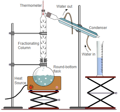
Ethanol (C₂H₅OH) can be separated from water (H₂O) through fractional distillation, leveraging their different boiling points. Ethanol boils at approximately 78°C, whereas water boils at 100°C under standard atmospheric pressure (1 atm). During distillation, the liquid mixture is heated, causing the lower-boiling components to vaporize at a faster rate than the higher-boiling components. The vapor rises through a fractionating column, where it undergoes multiple cycles of condensation and vaporization, increasing its purity before being sent through the condenser and collected in a receiving flask.

The process is governed by phase equilibrium, where the rates of evaporation and condensation reach a dynamic balance. The degree of separation can be influenced by temperature and pressure within the distillation column.

To investigate these factors, two experiments were conducted using a fractional distillation setup to analyze how varying temperature and pressure affect ethanol purity in the collected distillate. The setup used in the experiments is shown in Figure 1.

Figure 1.

Experiment 1

A mixture of ethanol and water was heated in the round-bottom flask, and the temperature at the top of the fractionating column was adjusted to achieve separation. The pressure was held at 1 atm (101.3 kPa). The condensate was collected in the receiving flask (a graduated cylinder) and analyzed for ethanol content.

Table 1.

Experiment 2

The pressure inside the distillation column was adjusted while keeping the temperature at 78°C, the boiling point of ethanol at 1 atm (101.3 kPa). The condensed fractions were collected and analyzed for ethanol concentration.

Table 2.

According to Table 1, at what temperature is the ethanol content 83%?

Item 14

Ethanol (C₂H₅OH) can be separated from water (H₂O) through fractional distillation, leveraging their different boiling points. Ethanol boils at approximately 78°C, whereas water boils at 100°C under standard atmospheric pressure (1 atm). During distillation, the liquid mixture is heated, causing the lower-boiling components to vaporize at a faster rate than the higher-boiling components. The vapor rises through a fractionating column, where it undergoes multiple cycles of condensation and vaporization, increasing its purity before being sent through the condenser and collected in a receiving flask.

The process is governed by phase equilibrium, where the rates of evaporation and condensation reach a dynamic balance. The degree of separation can be influenced by temperature and pressure within the distillation column.

To investigate these factors, two experiments were conducted using a fractional distillation setup to analyze how varying temperature and pressure affect ethanol purity in the collected distillate. The setup used in the experiments is shown in Figure 1.

Figure 1.

Experiment 1

A mixture of ethanol and water was heated in the round-bottom flask, and the temperature at the top of the fractionating column was adjusted to achieve separation. The pressure was held at 1 atm (101.3 kPa). The condensate was collected in the receiving flask (a graduated cylinder) and analyzed for ethanol content.

Table 1.

Experiment 2

The pressure inside the distillation column was adjusted while keeping the temperature at 78°C, the boiling point of ethanol at 1 atm (101.3 kPa). The condensed fractions were collected and analyzed for ethanol concentration.

Table 2.

At each temperature in Experiment 1, the purest ethanol vapor would most likely be found:

Item 15

Ethanol (C₂H₅OH) can be separated from water (H₂O) through fractional distillation, leveraging their different boiling points. Ethanol boils at approximately 78°C, whereas water boils at 100°C under standard atmospheric pressure (1 atm). During distillation, the liquid mixture is heated, causing the lower-boiling components to vaporize at a faster rate than the higher-boiling components. The vapor rises through a fractionating column, where it undergoes multiple cycles of condensation and vaporization, increasing its purity before being sent through the condenser and collected in a receiving flask.

The process is governed by phase equilibrium, where the rates of evaporation and condensation reach a dynamic balance. The degree of separation can be influenced by temperature and pressure within the distillation column.

To investigate these factors, two experiments were conducted using a fractional distillation setup to analyze how varying temperature and pressure affect ethanol purity in the collected distillate. The setup used in the experiments is shown in Figure 1.

Figure 1.

Experiment 1

A mixture of ethanol and water was heated in the round-bottom flask, and the temperature at the top of the fractionating column was adjusted to achieve separation. The pressure was held at 1 atm (101.3 kPa). The condensate was collected in the receiving flask (a graduated cylinder) and analyzed for ethanol content.

Table 1.

Experiment 2

The pressure inside the distillation column was adjusted while keeping the temperature at 78°C, the boiling point of ethanol at 1 atm (101.3 kPa). The condensed fractions were collected and analyzed for ethanol concentration.

Table 2.

During Experiment 1, an additional trial was conducted at 76°C, resulting in only 3% ethanol content in the receiving flask. Which of the following best explains why the separation was less effective at this temperature? 

Item 16

Ethanol (C₂H₅OH) can be separated from water (H₂O) through fractional distillation, leveraging their different boiling points. Ethanol boils at approximately 78°C, whereas water boils at 100°C under standard atmospheric pressure (1 atm). During distillation, the liquid mixture is heated, causing the lower-boiling components to vaporize at a faster rate than the higher-boiling components. The vapor rises through a fractionating column, where it undergoes multiple cycles of condensation and vaporization, increasing its purity before being sent through the condenser and collected in a receiving flask.

The process is governed by phase equilibrium, where the rates of evaporation and condensation reach a dynamic balance. The degree of separation can be influenced by temperature and pressure within the distillation column.

To investigate these factors, two experiments were conducted using a fractional distillation setup to analyze how varying temperature and pressure affect ethanol purity in the collected distillate. The setup used in the experiments is shown in Figure 1.

Figure 1.

Experiment 1

A mixture of ethanol and water was heated in the round-bottom flask, and the temperature at the top of the fractionating column was adjusted to achieve separation. The pressure was held at 1 atm (101.3 kPa). The condensate was collected in the receiving flask (a graduated cylinder) and analyzed for ethanol content.

Table 1.

Experiment 2

The pressure inside the distillation column was adjusted while keeping the temperature at 78°C, the boiling point of ethanol at 1 atm (101.3 kPa). The condensed fractions were collected and analyzed for ethanol concentration.

Table 2.

If an additional data point was recorded in Experiment 2 at a pressure of 50 kPa, what ethanol content would be expected in the receiving flask?

Item 17

Ethanol (C₂H₅OH) can be separated from water (H₂O) through fractional distillation, leveraging their different boiling points. Ethanol boils at approximately 78°C, whereas water boils at 100°C under standard atmospheric pressure (1 atm). During distillation, the liquid mixture is heated, causing the lower-boiling components to vaporize at a faster rate than the higher-boiling components. The vapor rises through a fractionating column, where it undergoes multiple cycles of condensation and vaporization, increasing its purity before being sent through the condenser and collected in a receiving flask.

The process is governed by phase equilibrium, where the rates of evaporation and condensation reach a dynamic balance. The degree of separation can be influenced by temperature and pressure within the distillation column.

To investigate these factors, two experiments were conducted using a fractional distillation setup to analyze how varying temperature and pressure affect ethanol purity in the collected distillate. The setup used in the experiments is shown in Figure 1.

Figure 1.

Experiment 1

A mixture of ethanol and water was heated in the round-bottom flask, and the temperature at the top of the fractionating column was adjusted to achieve separation. The pressure was held at 1 atm (101.3 kPa). The condensate was collected in the receiving flask (a graduated cylinder) and analyzed for ethanol content.

Table 1.

Experiment 2

The pressure inside the distillation column was adjusted while keeping the temperature at 78°C, the boiling point of ethanol at 1 atm (101.3 kPa). The condensed fractions were collected and analyzed for ethanol concentration.

Table 2.

What is the relationship between pressure and ethanol content as indicated in Table 2?

Item 18

Ethanol (C₂H₅OH) can be separated from water (H₂O) through fractional distillation, leveraging their different boiling points. Ethanol boils at approximately 78°C, whereas water boils at 100°C under standard atmospheric pressure (1 atm). During distillation, the liquid mixture is heated, causing the lower-boiling components to vaporize at a faster rate than the higher-boiling components. The vapor rises through a fractionating column, where it undergoes multiple cycles of condensation and vaporization, increasing its purity before being sent through the condenser and collected in a receiving flask.

The process is governed by phase equilibrium, where the rates of evaporation and condensation reach a dynamic balance. The degree of separation can be influenced by temperature and pressure within the distillation column.

To investigate these factors, two experiments were conducted using a fractional distillation setup to analyze how varying temperature and pressure affect ethanol purity in the collected distillate. The setup used in the experiments is shown in Figure 1.

Figure 1.

Experiment 1

A mixture of ethanol and water was heated in the round-bottom flask, and the temperature at the top of the fractionating column was adjusted to achieve separation. The pressure was held at 1 atm (101.3 kPa). The condensate was collected in the receiving flask (a graduated cylinder) and analyzed for ethanol content.

Table 1.

Experiment 2

The pressure inside the distillation column was adjusted while keeping the temperature at 78°C, the boiling point of ethanol at 1 atm (101.3 kPa). The condensed fractions were collected and analyzed for ethanol concentration.

Table 2.

Which of the following conclusions can be drawn from the combined results of Experiments 1 and 2?

Item 19

In the study of nuclear reactions, particularly in fusion processes, the concept of cross-section plays a crucial role. The cross-section (σ) of a nuclear reaction measures the likelihood of a particular interaction occurring between particles, analogous to how a larger target area increases the chance of hitting a dartboard. Cross-sections are often expressed in units of barns (1 barn = 10^-28) square meters).

Cross-sections are influenced by several factors, including the energy of the colliding particles, the type of nuclear reaction, and the nature of the interacting nuclei. Higher cross-sections generally indicate a greater probability of a reaction occurring, making them a key parameter in fusion research and nuclear reaction design.

One of the most important factors affecting cross-section is the incident energy (E) of the colliding particles. The incident energy refers to the kinetic energy of the incoming particle as it approaches the target nucleus. In the context of fusion, this is the energy with which two nuclei collide.

Figure 1 illustrates the variation of cross-section (σ) with incident energy (E) for two different fusion reactions:

Reaction 1 (Deuterium-Tritium Fusion): [latex]^{2}\!H+^{3}\!\!\!H \rightarrow\,^{4}\!He+n[/latex]

Reaction 2 (Helium-3 Fusion): [latex]^{3}\!He+^{3}\!\!\!He \rightarrow\,^{4}\!He+p+p[/latex]

Figure 1.

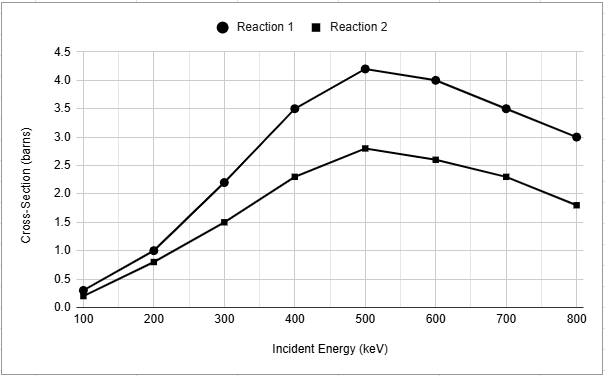
Table 1 depicts how the cross section (σ) varies with the relative velocity (v) of the colliding nuclei for the same fusion reactions. The velocity is given in units of 1000 km/s.

Table 1.

Based on the data, which incident energy value is associated with the greatest likelihood that an interaction will occur between two helium-3 particles?

Item 20

In the study of nuclear reactions, particularly in fusion processes, the concept of cross-section plays a crucial role. The cross-section (σ) of a nuclear reaction measures the likelihood of a particular interaction occurring between particles, analogous to how a larger target area increases the chance of hitting a dartboard. Cross-sections are often expressed in units of barns (1 barn = 10^-28) square meters).

Cross-sections are influenced by several factors, including the energy of the colliding particles, the type of nuclear reaction, and the nature of the interacting nuclei. Higher cross-sections generally indicate a greater probability of a reaction occurring, making them a key parameter in fusion research and nuclear reaction design.

One of the most important factors affecting cross-section is the incident energy (E) of the colliding particles. The incident energy refers to the kinetic energy of the incoming particle as it approaches the target nucleus. In the context of fusion, this is the energy with which two nuclei collide.

Figure 1 illustrates the variation of cross-section (σ) with incident energy (E) for two different fusion reactions:

Reaction 1 (Deuterium-Tritium Fusion): [latex]^{2}\!H+^{3}\!\!\!H \rightarrow\,^{4}\!He+n[/latex]

Reaction 2 (Helium-3 Fusion): [latex]^{3}\!He+^{3}\!\!\!He \rightarrow\,^{4}\!He+p+p[/latex]

Figure 1.

Table 1 depicts how the cross section (σ) varies with the relative velocity (v) of the colliding nuclei for the same fusion reactions. The velocity is given in units of 1000 km/s.

Table 1.

According to Figure 1, how does the cross-section for the deuterium-tritium (D-T) reaction compare to that of the helium-3 (He-3) reaction at an incident energy of 600 keV?

Item 21

In the study of nuclear reactions, particularly in fusion processes, the concept of cross-section plays a crucial role. The cross-section (σ) of a nuclear reaction measures the likelihood of a particular interaction occurring between particles, analogous to how a larger target area increases the chance of hitting a dartboard. Cross-sections are often expressed in units of barns (1 barn = 10^-28) square meters).

Cross-sections are influenced by several factors, including the energy of the colliding particles, the type of nuclear reaction, and the nature of the interacting nuclei. Higher cross-sections generally indicate a greater probability of a reaction occurring, making them a key parameter in fusion research and nuclear reaction design.

One of the most important factors affecting cross-section is the incident energy (E) of the colliding particles. The incident energy refers to the kinetic energy of the incoming particle as it approaches the target nucleus. In the context of fusion, this is the energy with which two nuclei collide.

Figure 1 illustrates the variation of cross-section (σ) with incident energy (E) for two different fusion reactions:

Reaction 1 (Deuterium-Tritium Fusion): [latex]^{2}\!H+^{3}\!\!\!H \rightarrow\,^{4}\!He+n[/latex]

Reaction 2 (Helium-3 Fusion): [latex]^{3}\!He+^{3}\!\!\!He \rightarrow\,^{4}\!He+p+p[/latex]

Figure 1.

Table 1 depicts how the cross section (σ) varies with the relative velocity (v) of the colliding nuclei for the same fusion reactions. The velocity is given in units of 1000 km/s.

Table 1.

Assume a direct relationship between cross section and the efficiency of a nuclear fusion reaction. At a relative velocity of 3,000 km/s, what can be inferred about the efficiency of D-T fusion compared to that of He-3 fusion?

Item 22

In the study of nuclear reactions, particularly in fusion processes, the concept of cross-section plays a crucial role. The cross-section (σ) of a nuclear reaction measures the likelihood of a particular interaction occurring between particles, analogous to how a larger target area increases the chance of hitting a dartboard. Cross-sections are often expressed in units of barns (1 barn = 10^-28) square meters).

Cross-sections are influenced by several factors, including the energy of the colliding particles, the type of nuclear reaction, and the nature of the interacting nuclei. Higher cross-sections generally indicate a greater probability of a reaction occurring, making them a key parameter in fusion research and nuclear reaction design.

One of the most important factors affecting cross-section is the incident energy (E) of the colliding particles. The incident energy refers to the kinetic energy of the incoming particle as it approaches the target nucleus. In the context of fusion, this is the energy with which two nuclei collide.

Figure 1 illustrates the variation of cross-section (σ) with incident energy (E) for two different fusion reactions:

Reaction 1 (Deuterium-Tritium Fusion): [latex]^{2}\!H+^{3}\!\!\!H \rightarrow\,^{4}\!He+n[/latex]

Reaction 2 (Helium-3 Fusion): [latex]^{3}\!He+^{3}\!\!\!He \rightarrow\,^{4}\!He+p+p[/latex]

Figure 1.

Table 1 depicts how the cross section (σ) varies with the relative velocity (v) of the colliding nuclei for the same fusion reactions. The velocity is given in units of 1000 km/s.

Table 1.

A researcher proposes studying the tritium-tritium (T-T) reaction, hypothesizing that it follows a cross-section trend somewhere between reaction 1 and reaction 2. What relative velocity is most likely to produce the peak cross-section value of the T-T reaction?

Item 23

In the study of nuclear reactions, particularly in fusion processes, the concept of cross-section plays a crucial role. The cross-section (σ) of a nuclear reaction measures the likelihood of a particular interaction occurring between particles, analogous to how a larger target area increases the chance of hitting a dartboard. Cross-sections are often expressed in units of barns (1 barn = 10^-28) square meters).

Cross-sections are influenced by several factors, including the energy of the colliding particles, the type of nuclear reaction, and the nature of the interacting nuclei. Higher cross-sections generally indicate a greater probability of a reaction occurring, making them a key parameter in fusion research and nuclear reaction design.

One of the most important factors affecting cross-section is the incident energy (E) of the colliding particles. The incident energy refers to the kinetic energy of the incoming particle as it approaches the target nucleus. In the context of fusion, this is the energy with which two nuclei collide.

Figure 1 illustrates the variation of cross-section (σ) with incident energy (E) for two different fusion reactions:

Reaction 1 (Deuterium-Tritium Fusion): [latex]^{2}\!H+^{3}\!\!\!H \rightarrow\,^{4}\!He+n[/latex]

Reaction 2 (Helium-3 Fusion): [latex]^{3}\!He+^{3}\!\!\!He \rightarrow\,^{4}\!He+p+p[/latex]

Figure 1.

Table 1 depicts how the cross section (σ) varies with the relative velocity (v) of the colliding nuclei for the same fusion reactions. The velocity is given in units of 1000 km/s.

Table 1.

A student studying the effect of incident energy on cross sections for various fusion reactions had predicted exponential growth in cross section as incident energy increased, since a higher kinetic energy of colliding particles should lead to more interaction between particles. However, the data in Figure 1 does not match this prediction. What could be a possible explanation for this?

Item 24

Scientists conducted two studies to investigate how ocean depth affects the composition of sediments found on the seafloor. They analyzed different sediment samples collected from varying depths in the ocean.

Study 1

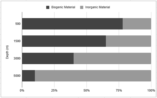
A research team collected sediment samples from four different depths in the Pacific Ocean: 500 m, 1,500 m, 3,000 m, and 5,000 m. They measured the percentage of the sediment that was composed of biogenic material (organic remains from marine organisms) and inorganic material (minerals and rock fragments). The results are shown in Figure 1.

Figure 1.

Study 2

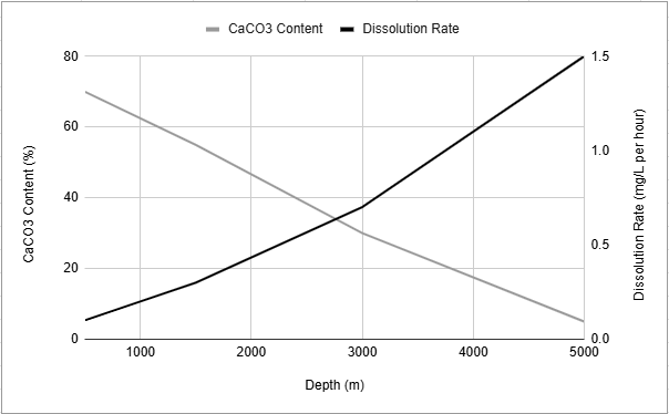
Another research team analyzed the calcium carbonate (CaCO₃) content of the sediments at depths up to 5000m. Calcium carbonate is a major component of marine organisms such as shells and coral. The scientists also measured the dissolution rate (how quickly calcium carbonate dissolves into the water) at each depth. Their findings are shown in Figure 2.

Knowing the calcium carbonate content of the sediments and the dissolution rate at different depths can help scientists determine the carbonate compensation depth (CCD), or the depth in the ocean where the rate of calcium carbonate dissolution equals the rate of its deposition. Below this depth, calcium carbonate dissolves faster than it accumulates, meaning very little or no calcium carbonate is found in the sediments.

Figure 2.

According to Figure 1, at what depth is the percentage of inorganic material approximately 35%?

Item 25

Scientists conducted two studies to investigate how ocean depth affects the composition of sediments found on the seafloor. They analyzed different sediment samples collected from varying depths in the ocean.

Study 1

A research team collected sediment samples from four different depths in the Pacific Ocean: 500 m, 1,500 m, 3,000 m, and 5,000 m. They measured the percentage of the sediment that was composed of biogenic material (organic remains from marine organisms) and inorganic material (minerals and rock fragments). The results are shown in Figure 1.

Figure 1.

Study 2

Another research team analyzed the calcium carbonate (CaCO₃) content of the sediments at depths up to 5000m. Calcium carbonate is a major component of marine organisms such as shells and coral. The scientists also measured the dissolution rate (how quickly calcium carbonate dissolves into the water) at each depth. Their findings are shown in Figure 2.

Knowing the calcium carbonate content of the sediments and the dissolution rate at different depths can help scientists determine the carbonate compensation depth (CCD), or the depth in the ocean where the rate of calcium carbonate dissolution equals the rate of its deposition. Below this depth, calcium carbonate dissolves faster than it accumulates, meaning very little or no calcium carbonate is found in the sediments.

Figure 2.

Assuming a linear relationship between percentage of inorganic and biogenic materials and depth, at what depth would it be reasonable to expect equal percentages of biogenic and inorganic materials?

Item 26

Scientists conducted two studies to investigate how ocean depth affects the composition of sediments found on the seafloor. They analyzed different sediment samples collected from varying depths in the ocean.

Study 1

A research team collected sediment samples from four different depths in the Pacific Ocean: 500 m, 1,500 m, 3,000 m, and 5,000 m. They measured the percentage of the sediment that was composed of biogenic material (organic remains from marine organisms) and inorganic material (minerals and rock fragments). The results are shown in Figure 1.

Figure 1.

Study 2

Another research team analyzed the calcium carbonate (CaCO₃) content of the sediments at depths up to 5000m. Calcium carbonate is a major component of marine organisms such as shells and coral. The scientists also measured the dissolution rate (how quickly calcium carbonate dissolves into the water) at each depth. Their findings are shown in Figure 2.

Knowing the calcium carbonate content of the sediments and the dissolution rate at different depths can help scientists determine the carbonate compensation depth (CCD), or the depth in the ocean where the rate of calcium carbonate dissolution equals the rate of its deposition. Below this depth, calcium carbonate dissolves faster than it accumulates, meaning very little or no calcium carbonate is found in the sediments.

Figure 2.

According to the results of Study 2, what depth is likely closest to the carbonate compensation depth (CCD)?

Item 27

Scientists conducted two studies to investigate how ocean depth affects the composition of sediments found on the seafloor. They analyzed different sediment samples collected from varying depths in the ocean.

Study 1

A research team collected sediment samples from four different depths in the Pacific Ocean: 500 m, 1,500 m, 3,000 m, and 5,000 m. They measured the percentage of the sediment that was composed of biogenic material (organic remains from marine organisms) and inorganic material (minerals and rock fragments). The results are shown in Figure 1.

Figure 1.

Study 2

Another research team analyzed the calcium carbonate (CaCO₃) content of the sediments at depths up to 5000m. Calcium carbonate is a major component of marine organisms such as shells and coral. The scientists also measured the dissolution rate (how quickly calcium carbonate dissolves into the water) at each depth. Their findings are shown in Figure 2.

Knowing the calcium carbonate content of the sediments and the dissolution rate at different depths can help scientists determine the carbonate compensation depth (CCD), or the depth in the ocean where the rate of calcium carbonate dissolution equals the rate of its deposition. Below this depth, calcium carbonate dissolves faster than it accumulates, meaning very little or no calcium carbonate is found in the sediments.

Figure 2.

A scientist hypothesizes that increasing pressure could contribute to an increase in the dissolution rate of calcium carbonate. Does the data support this hypothesis?

Item 28

Scientists conducted two studies to investigate how ocean depth affects the composition of sediments found on the seafloor. They analyzed different sediment samples collected from varying depths in the ocean.

Study 1

A research team collected sediment samples from four different depths in the Pacific Ocean: 500 m, 1,500 m, 3,000 m, and 5,000 m. They measured the percentage of the sediment that was composed of biogenic material (organic remains from marine organisms) and inorganic material (minerals and rock fragments). The results are shown in Figure 1.

Figure 1.

Study 2

Another research team analyzed the calcium carbonate (CaCO₃) content of the sediments at depths up to 5000m. Calcium carbonate is a major component of marine organisms such as shells and coral. The scientists also measured the dissolution rate (how quickly calcium carbonate dissolves into the water) at each depth. Their findings are shown in Figure 2.

Knowing the calcium carbonate content of the sediments and the dissolution rate at different depths can help scientists determine the carbonate compensation depth (CCD), or the depth in the ocean where the rate of calcium carbonate dissolution equals the rate of its deposition. Below this depth, calcium carbonate dissolves faster than it accumulates, meaning very little or no calcium carbonate is found in the sediments.

Figure 2.

Which of the following factors most likely contributes to the decrease in biogenic material at greater depths?

Item 29

Scientists conducted two studies to investigate how ocean depth affects the composition of sediments found on the seafloor. They analyzed different sediment samples collected from varying depths in the ocean.

Study 1

A research team collected sediment samples from four different depths in the Pacific Ocean: 500 m, 1,500 m, 3,000 m, and 5,000 m. They measured the percentage of the sediment that was composed of biogenic material (organic remains from marine organisms) and inorganic material (minerals and rock fragments). The results are shown in Figure 1.

Figure 1.

Study 2

Another research team analyzed the calcium carbonate (CaCO₃) content of the sediments at depths up to 5000m. Calcium carbonate is a major component of marine organisms such as shells and coral. The scientists also measured the dissolution rate (how quickly calcium carbonate dissolves into the water) at each depth. Their findings are shown in Figure 2.

Knowing the calcium carbonate content of the sediments and the dissolution rate at different depths can help scientists determine the carbonate compensation depth (CCD), or the depth in the ocean where the rate of calcium carbonate dissolution equals the rate of its deposition. Below this depth, calcium carbonate dissolves faster than it accumulates, meaning very little or no calcium carbonate is found in the sediments.

Figure 2.

Which of the following statements best explains the relationship between ocean depth, biogenic material content, and calcium carbonate content?

Item 30

A group of scientists conducted three experiments to examine how temperature and concentration affect the rate of a chemical reaction. They studied the reaction between magnesium metal (Mg) and hydrochloric acid (HCl), which produces magnesium chloride (MgCl₂) and hydrogen gas (H₂) according to the following equation:

Mg (s) + 2HCl (aq) [latex]\rightarrow[/latex] MgCl₂ (aq) + H₂ (g)

Experiment 1

The scientists conducted the reaction at five different temperatures (10°C, 25°C, 50°C, 75°C, and 100°C) while keeping the concentration of HCl constant at 1.0 M. The results are shown in Table 1.

Table 1.

Experiment 2

The scientists varied the concentration of HCl from 0.25M to 2.5M while keeping the temperature constant at 25°C. The results are displayed in Table 2.

Table 2.

Experiment 3

The scientists tested the reaction at different combinations of temperature and concentration to observe their combined effect. The results are shown in Table 3.

Table 3.

Based on the results of Experiment 1, what is the relationship between temperature and reaction rate?

Item 31

A group of scientists conducted three experiments to examine how temperature and concentration affect the rate of a chemical reaction. They studied the reaction between magnesium metal (Mg) and hydrochloric acid (HCl), which produces magnesium chloride (MgCl₂) and hydrogen gas (H₂) according to the following equation:

Mg (s) + 2HCl (aq) [latex]\rightarrow[/latex] MgCl₂ (aq) + H₂ (g)

Experiment 1

The scientists conducted the reaction at five different temperatures (10°C, 25°C, 50°C, 75°C, and 100°C) while keeping the concentration of HCl constant at 1.0 M. The results are shown in Table 1.

Table 1.

Experiment 2

The scientists varied the concentration of HCl from 0.25M to 2.5M while keeping the temperature constant at 25°C. The results are displayed in Table 2.

Table 2.

Experiment 3

The scientists tested the reaction at different combinations of temperature and concentration to observe their combined effect. The results are shown in Table 3.

Table 3.

A scientist ran the reaction at 25°C and recorded a time of 55 seconds for Mg to dissolve and 24.6 mL of H₂ gas produced per minute. The concentration of HCl used in this trial was most likely between:

Item 32

A group of scientists conducted three experiments to examine how temperature and concentration affect the rate of a chemical reaction. They studied the reaction between magnesium metal (Mg) and hydrochloric acid (HCl), which produces magnesium chloride (MgCl₂) and hydrogen gas (H₂) according to the following equation:

Mg (s) + 2HCl (aq) [latex]\rightarrow[/latex] MgCl₂ (aq) + H₂ (g)

Experiment 1

The scientists conducted the reaction at five different temperatures (10°C, 25°C, 50°C, 75°C, and 100°C) while keeping the concentration of HCl constant at 1.0 M. The results are shown in Table 1.

Table 1.

Experiment 2

The scientists varied the concentration of HCl from 0.25M to 2.5M while keeping the temperature constant at 25°C. The results are displayed in Table 2.

Table 2.

Experiment 3

The scientists tested the reaction at different combinations of temperature and concentration to observe their combined effect. The results are shown in Table 3.

Table 3.

Based on the data collected in Experiment 3, which factor–HCl concentration or reaction temperature–has a greater effect on reaction rate?

Item 33

A group of scientists conducted three experiments to examine how temperature and concentration affect the rate of a chemical reaction. They studied the reaction between magnesium metal (Mg) and hydrochloric acid (HCl), which produces magnesium chloride (MgCl₂) and hydrogen gas (H₂) according to the following equation:

Mg (s) + 2HCl (aq) [latex]\rightarrow[/latex] MgCl₂ (aq) + H₂ (g)

Experiment 1

The scientists conducted the reaction at five different temperatures (10°C, 25°C, 50°C, 75°C, and 100°C) while keeping the concentration of HCl constant at 1.0 M. The results are shown in Table 1.

Table 1.

Experiment 2

The scientists varied the concentration of HCl from 0.25M to 2.5M while keeping the temperature constant at 25°C. The results are displayed in Table 2.

Table 2.

Experiment 3

The scientists tested the reaction at different combinations of temperature and concentration to observe their combined effect. The results are shown in Table 3.

Table 3.

If the reaction was run at 75°C with 2.0 M HCl, what would be reasonable values for the time it takes for Mg to dissolve and the amount of H₂ gas produced?

Item 34

A group of scientists conducted three experiments to examine how temperature and concentration affect the rate of a chemical reaction. They studied the reaction between magnesium metal (Mg) and hydrochloric acid (HCl), which produces magnesium chloride (MgCl₂) and hydrogen gas (H₂) according to the following equation:

Mg (s) + 2HCl (aq) [latex]\rightarrow[/latex] MgCl₂ (aq) + H₂ (g)

Experiment 1

The scientists conducted the reaction at five different temperatures (10°C, 25°C, 50°C, 75°C, and 100°C) while keeping the concentration of HCl constant at 1.0 M. The results are shown in Table 1.

Table 1.

Experiment 2

The scientists varied the concentration of HCl from 0.25M to 2.5M while keeping the temperature constant at 25°C. The results are displayed in Table 2.

Table 2.

Experiment 3

The scientists tested the reaction at different combinations of temperature and concentration to observe their combined effect. The results are shown in Table 3.

Table 3.

Which graph most accurately represents the effect of HCl concentration and temperature on the time it takes for Mg to dissolve in the reaction?

Item 35

A group of scientists conducted three experiments to examine how temperature and concentration affect the rate of a chemical reaction. They studied the reaction between magnesium metal (Mg) and hydrochloric acid (HCl), which produces magnesium chloride (MgCl₂) and hydrogen gas (H₂) according to the following equation:

Mg (s) + 2HCl (aq) [latex]\rightarrow[/latex] MgCl₂ (aq) + H₂ (g)

Experiment 1

The scientists conducted the reaction at five different temperatures (10°C, 25°C, 50°C, 75°C, and 100°C) while keeping the concentration of HCl constant at 1.0 M. The results are shown in Table 1.

Table 1.

Experiment 2

The scientists varied the concentration of HCl from 0.25M to 2.5M while keeping the temperature constant at 25°C. The results are displayed in Table 2.

Table 2.

Experiment 3

The scientists tested the reaction at different combinations of temperature and concentration to observe their combined effect. The results are shown in Table 3.

Table 3.

Which statement best explains how the temperature affects the reaction rate?

Item 36

Scientists conducted research to understand the effects of temperature and salinity on the hatching success and growth of shrimp larvae. Newly hatched larvae of Species X and Species Y were exposed to one of 12 different conditions (Conditions 1–12) for 14 days, and then their growth was measured. Conditions 1–12 varied only in temperature and/or salinity. Table 1 displays the average length of the larvae for each species under each condition. Figure 1 shows the average survival rate and average weight of the larvae of each species under Conditions 1–4.

Table 1.

*ppt = parts per thousand

Figure 1. 

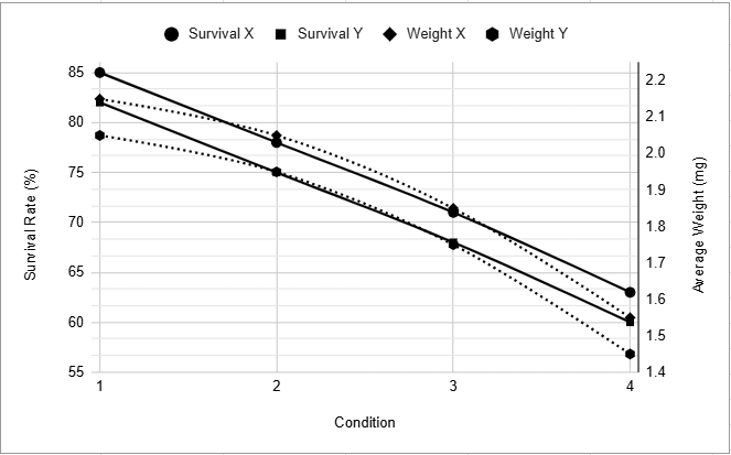
Based on the data in Table 1, how did the average length of Species X larvae change as the temperature increased from 20°C to 30°C at a salinity of 15 ppt?

Item 37

Scientists conducted research to understand the effects of temperature and salinity on the hatching success and growth of shrimp larvae. Newly hatched larvae of Species X and Species Y were exposed to one of 12 different conditions (Conditions 1–12) for 14 days, and then their growth was measured. Conditions 1–12 varied only in temperature and/or salinity. Table 1 displays the average length of the larvae for each species under each condition. Figure 1 shows the average survival rate and average weight of the larvae of each species under Conditions 1–4.

Table 1.

*ppt = parts per thousand

Figure 1. 

At each Condition 1-4, how do the average length, average weight, and survival rate of Species X compare to those of Species Y?

Item 38

Scientists conducted research to understand the effects of temperature and salinity on the hatching success and growth of shrimp larvae. Newly hatched larvae of Species X and Species Y were exposed to one of 12 different conditions (Conditions 1–12) for 14 days, and then their growth was measured. Conditions 1–12 varied only in temperature and/or salinity. Table 1 displays the average length of the larvae for each species under each condition. Figure 1 shows the average survival rate and average weight of the larvae of each species under Conditions 1–4.

Table 1.

*ppt = parts per thousand

Figure 1. 

Considering Table 1 and Figure 1, what is the relationship between salinity and average weight of Species Y larvae at 20°C?

Item 39

Scientists conducted research to understand the effects of temperature and salinity on the hatching success and growth of shrimp larvae. Newly hatched larvae of Species X and Species Y were exposed to one of 12 different conditions (Conditions 1–12) for 14 days, and then their growth was measured. Conditions 1–12 varied only in temperature and/or salinity. Table 1 displays the average length of the larvae for each species under each condition. Figure 1 shows the average survival rate and average weight of the larvae of each species under Conditions 1–4.

Table 1.

*ppt = parts per thousand

Figure 1. 

If a new condition was tested with a temperature of 20°C and a salinity of 10 ppt, what would be the most likely survival rate for Species X?

Item 40

Scientists conducted research to understand the effects of temperature and salinity on the hatching success and growth of shrimp larvae. Newly hatched larvae of Species X and Species Y were exposed to one of 12 different conditions (Conditions 1–12) for 14 days, and then their growth was measured. Conditions 1–12 varied only in temperature and/or salinity. Table 1 displays the average length of the larvae for each species under each condition. Figure 1 shows the average survival rate and average weight of the larvae of each species under Conditions 1–4.

Table 1.

*ppt = parts per thousand

Figure 1. 

Given that the optimal salinity for hatching success of Species X larvae is 5 ppt, how many conditions provided a salinity that was higher than the optimal level?